Deep Learning Development Environment Setup Guide

Deep Learning is a branch of artificial intelligence (AI) that excels in analyzing complex data and learning patterns. In this post, we’ll cover the basics of deep learning, explore real-world applications, and guide you through setting up a development environment. This will help beginners get started with deep learning and understand its practical applications.

Table of Contents

1. Deep Learning Overview

Deep learning is based on Artificial Neural Networks (ANNs), where multiple layers of neurons interact to process data. Key deep learning models include:

Convolutional Neural Networks (CNNs): Primarily used for image processing. CNNs are effective at extracting features from images and are widely used in applications such as self-driving cars and facial recognition.
Recurrent Neural Networks (RNNs): Suitable for sequential data or natural language processing. RNNs use the output of the previous step as input for the next step, making them powerful for tasks like translation and speech recognition.
Transformers: Excel at handling complex data like natural language processing. Transformer models, known for their parallel processing capabilities, include popular examples like the GPT series.

Deep learning models are applied across various industries. For instance, AlphaGo outperformed human players in the game of Go,

2. Current Deep Learning Capabilities

The advancements in deep learning technology are remarkable. MidJourney AI won a Colorado state art competition, showcasing its sophisticated image generation capabilities, while Chat-GPT can create complex educational curricula. These technologies have evolved from simple models to practical tools for solving complex problems.

AI technologies for audio data processing have also advanced, enabling applications like voice style transfer using famous singers’ voices. Photoshop AI offers innovative features for image creation and editing, enhancing user creativity.

3. Setting Up a Deep Learning Development Environment

To start with deep learning, it’s crucial to set up the appropriate development environment. We will cover both Google Colab and Anaconda to help you get started.

1) Google Colab

Google Colab is a cloud-based, free Jupyter notebook environment that requires no installation. It supports GPU acceleration for fast computations and provides a consistent setup across devices.

Go to the Google Colab page.
Sign in with your Google account.
Create a new notebook and start running Python code instantly.

2) Anaconda Installation and Setup

Anaconda provides a local, Python-based data science platform that makes it easy to manage and install various libraries. You can run deep learning models locally by setting up TensorFlow, Keras, Pandas, and other necessary libraries.

Steps to Download and Install Anaconda:

Download Anaconda:

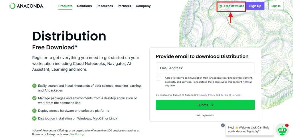
Visit the Anaconda official website.
Click the “Download” button on the page.
Select the installer that matches your operating system.

Install Anaconda:

Once the download is complete, run the installer.
Click “Next” to start the installation.
Choose the installation path or use the default path.
Check the “Add Anaconda to my PATH environment variable” option and click “Install.”
- While not mandatory, this option allows you to easily use Anaconda from the command prompt.
Click “Finish” once the installation is complete.

Set Up Anaconda Environment:

After installation, launch the “Anaconda Prompt.”
- On Windows, click the “Start” button, search for “Anaconda Prompt,” and launch it.
Use the following commands to create a virtual environment and install the necessary libraries.

   # Create and activate a virtual environment
   conda create -n tensorflow python=3.9 ipykernel
   activate tensorflow

   # Install required libraries
   conda install tensorflow keras notebook ipykernel

Navigate to your working directory and launch Jupyter Notebook.

   # Navigate to your workspace
   cd C:\workspace

   # Launch Jupyter Notebook
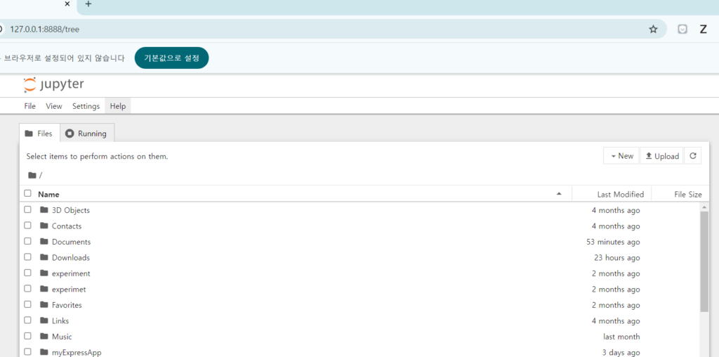
   jupyter notebook

Jupyter Notebook will open automatically in your web browser, where you can start writing and executing Python code.

4. Handwritten Digit Classification Example

To understand the basic concepts of deep learning, let’s walk through a handwritten digit classification example using the MNIST dataset. This example involves the following steps:

Loading and Preprocessing Data: Load handwritten digit images, split them into training and test sets, and preprocess them.

   import numpy as np
   import pandas as pd
   from sklearn.model_selection import train_test_split
   from tensorflow.keras import utils

   # Load MNIST dataset
   mnist_csv = pd.read_csv('./dataset/mnist_train.csv', header=None, skiprows=1).values

   # Split data
   train, test = train_test_split(mnist_csv, test_size=0.3, random_state=1)
   X_train, Y_train = train[:, 1:], train[:, 0]
   X_test, Y_test = test[:, 1:], test[:, 0]

   # Convert labels to categorical format
   Y_train_cat = utils.to_categorical(Y_train)
   Y_test_cat = utils.to_categorical(Y_test)

Designing an MLP Model: Create a multilayer perceptron (MLP) neural network to classify the handwritten digits.

   from tensorflow.keras.layers import Input, Dense
   from tensorflow.keras.models import Model

   # Design MLP model
   mlp_input = Input(shape=(784,))
   h = Dense(256, activation='tanh')(mlp_input)
   h = Dense(128, activation='tanh')(h)
   mlp_output = Dense(10, activation='softmax')(h)

   mlp_model = Model(mlp_input, mlp_output)
   mlp_model.compile(loss='categorical_crossentropy', optimizer='adam', metrics=['accuracy'])
   mlp_model.summary()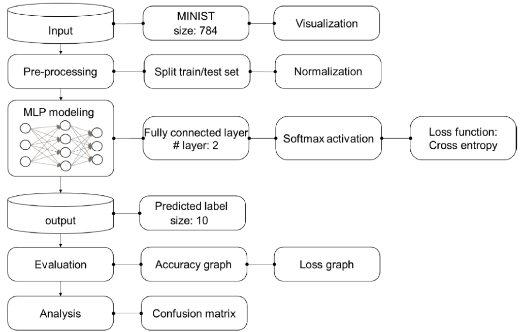

Training the Model: Visualize the training curves and evaluate the model’s performance.

   # Train the model
   model_history = mlp_model.fit(X_train, Y_train_cat, validation_data=(X_test, Y_test_cat), epochs=100, batch_size=256, shuffle=True, verbose=2)

   # Visualize training curves
   import matplotlib.pyplot as plt

   plt.plot(model_history.history['loss'])
   plt.plot(model_history.history['val_loss'])
   plt.xlabel('epochs'), plt.ylabel('Loss')
   plt.legend(['Train', 'Test'])
   plt.show()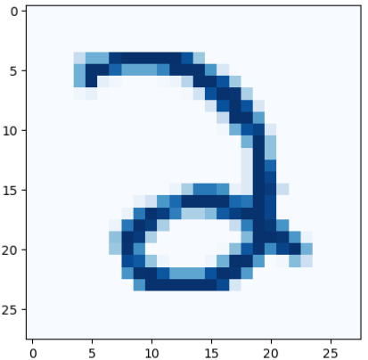

Evaluating Accuracy and Confusion Matrix: Analyze the classification results using accuracy, precision, recall, and visualize the confusion matrix.

   from sklearn.metrics import confusion_matrix
   import numpy as np

   # Visualize confusion matrix
   Y_test_cat_hat = mlp_model.predict(X_test)
   Y_test_hat = np.argmax(Y_test_cat_hat, axis=1)

   print(confusion_matrix(Y_test_hat, Y_test))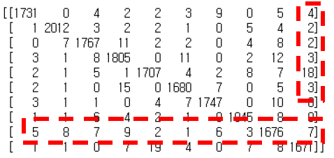

By following these steps, you can understand the structure and training process of a deep learning model.

Conclusion

Deep learning has established itself as a powerful tool for solving complex problems. In this post, we covered the basics of deep learning, set up a development environment, and walked through a practical example. We hope this guide helps you dive deeper into deep learning and explore its various applications.

If you found this post helpful, please subscribe and like it. We regularly provide more deep learning content!

This post is optimized for Google SEO, with relevant images and example code provided to help readers understand the concepts visually and practically.