In our previous post, we explored the basics of deep learning and set up a development environment using Google Colab and Anaconda. Now, it’s time to dive deeper into how we can apply this knowledge to a practical project. In this post, we’ll guide you step-by-step on how to build a simple neural network to classify handwritten digits using the MNIST dataset.
1. Understanding the Problem: Handwritten Digit Classification
The goal of this project is to create a model that can accurately classify handwritten digits (0-9) from images. We’ll use the MNIST dataset, which is a collection of 42,000 labeled images of handwritten numbers, each of size 28×28 pixels. These images contain various levels of intra-class variance and inter-class correlation, making this a great dataset for training a neural network.
Example of MNIST images:

Each image is labeled with a digit between 0 and 9, and our task is to build a model that can predict these labels based on the pixel data.
2. Loading and Preprocessing the Data
To start, we need to load the MNIST dataset and preprocess it for our model.
import numpy as np
import pandas as pd
from sklearn.model_selection import train_test_split
from tensorflow.keras import utils

# Load the MNIST dataset
mnist_csv = pd.read_csv('./dataset/mnist_train.csv', header=None, skiprows=1).values

# Split the dataset into training and testing sets
train, test = train_test_split(mnist_csv, test_size=0.3, random_state=1)
X_train, Y_train = train[:, 1:], train[:, 0]
X_test, Y_test = test[:, 1:], test[:, 0]

# Convert labels to one-hot vectors
Y_train_cat = utils.to_categorical(Y_train)
Y_test_cat = utils.to_categorical(Y_test)
What is one-hot encoding?
One-hot encoding is a way to convert categorical labels (like our digit labels) into a format that can be used by the neural network. For example, if a digit is 3, one-hot encoding will represent it as [0, 0, 0, 1, 0, 0, 0, 0, 0, 0].
3. Normalizing and Visualizing the Data
Before feeding the data into the model, it’s essential to normalize it. Normalization scales the pixel values (which range from 0 to 255) to a range between 0 and 1, making the model training more efficient.
# Normalize the dataset
X_train_norm = X_train / 255.0
X_test_norm = X_test / 255.0

# Visualize one of the training images
import matplotlib.pyplot as plt
import numpy as np

plt.imshow(np.reshape(X_train_norm[0], (28, 28)), cmap=plt.cm.Blues)
plt.show()
Why normalize?
Normalization helps improve the performance and stability of the neural network by ensuring that the input values are within a similar range.
4. Building the Neural Network Model
Now, let’s build a simple Multilayer Perceptron (MLP) model using Keras. Our model will have two hidden layers with ReLU activation functions, which are widely used due to their efficiency and ability to avoid certain training issues.
from tensorflow.keras.models import Sequential
from tensorflow.keras.layers import Dense

# Build the MLP model
mlp_model = Sequential()
mlp_model.add(Dense(512, activation='relu', input_shape=(784,)))
mlp_model.add(Dense(256, activation='relu'))
mlp_model.add(Dense(10, activation='softmax'))

mlp_model.summary()
Understanding the layers:
- Input layer: Takes in the flattened 784-pixel input.
- Hidden layers: Two layers with 512 and 256 units, using ReLU activation.
- Output layer: 10 units with softmax activation, corresponding to the digit classes (0-9).
5. Compiling and Training the Model
Next, we need to compile the model. We’ll use categorical cross-entropy as the loss function and Stochastic Gradient Descent (SGD) as the optimizer.
from tensorflow.keras.optimizers import SGD

# Compile the model
sgd = SGD(lr=0.005)
mlp_model.compile(loss='categorical_crossentropy', optimizer=sgd, metrics=['accuracy'])

# Train the model
model_history = mlp_model.fit(X_train_norm, Y_train_cat, epochs=15, batch_size=256, verbose=2, validation_data=(X_test_norm, Y_test_cat), shuffle=True)
Training the model:
During training, the model adjusts its weights based on the loss function to improve accuracy. This is done through multiple epochs, where each epoch represents one full pass through the entire training dataset.
6. Evaluating Model Performance
After training, it’s important to evaluate the model’s performance using the test data. We’ll visualize the loss and accuracy over the training epochs.
# Plot the loss curve
plt.plot(model_history.history['loss'])
plt.plot(model_history.history['val_loss'])
plt.title('Model Loss')
plt.ylabel('Loss')
plt.xlabel('Epoch')
plt.legend(['Train', 'Test'], loc='right')
plt.show()

# Plot the accuracy curve
plt.plot(model_history.history['accuracy'])
plt.plot(model_history.history['val_accuracy'])
plt.title('Model Accuracy')
plt.ylabel('Accuracy')
plt.xlabel('Epoch')
plt.legend(['Train', 'Test'], loc='right')
plt.show()
What do these curves tell us?
- Loss curve: Shows how the loss decreases with each epoch, indicating how well the model is learning.
- Accuracy curve: Shows the model’s accuracy over time, helping us understand its performance on both the training and testing data.
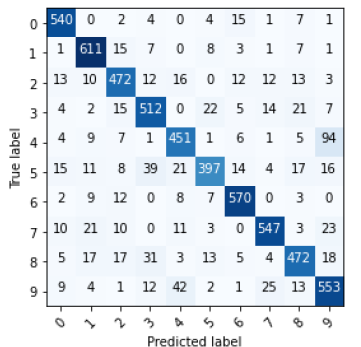
7. Analyzing Errors with a Confusion Matrix
To further analyze the model’s performance, we can use a confusion matrix. This will help us understand where the model is making mistakes and how often it confuses different digits.
from sklearn.metrics import confusion_matrix
import itertools

# Confusion matrix function
def plot_confusion_matrix(model_input, feature, label, class_info):
    pred=model_input.predict(feature)
    cnf_matrix=confusion_matrix(np.argmax(label,axis=1),np.argmax(pred,axis=1))
    plt.figure()
    plt.imshow(cnf_matrix,interpolation='nearest',cmap=plt.cm.Blues)
    tick_marks= np.arange(len(class_info))
    plt.xticks(tick_marks,class_info,rotation=45)
    plt.yticks(tick_marks,class_info)
    thresh=cnf_matrix.max()/2.
    for i, j in itertools.product(range(cnf_matrix.shape[0]), range(cnf_matrix.shape[1])):
         plt.text(j, i, cnf_matrix[i, j], horizontalalignment="center", color="white"
         if cnf_matrix[i, j] > thresh else "black")
    plt.tight_layout()
    plt.ylabel('True label')
    plt.xlabel('Predicted label')
    plt.show()

# Plot the confusion matrix
label = ['0','1','2','3','4','5','6','7','8','9']
plot_confusion_matrix(mlp_model, X_test_norm, Y_test_cat, class_info=label)
What is a confusion matrix?

A confusion matrix is a table that shows the number of correct and incorrect predictions made by the model for each class. It helps in identifying specific digits that the model may struggle with.
Conclusion
In this post, we’ve walked through the process of building, training, and evaluating a neural network to classify handwritten digits. By understanding each step—from data preprocessing to model evaluation—you can now create your own deep learning models for various tasks.
As you continue your journey, remember that practice and experimentation are key to mastering deep learning. Don’t hesitate to try different architectures, optimizers, and datasets to see how they impact your model’s performance.
Stay tuned for more posts where we’ll dive deeper into advanced techniques and strategies to further improve your deep learning models!
If you found this guide helpful, be sure to subscribe for more deep learning tutorials. Feel free to leave any questions or comments below!